Crystal Instruments SPIDER20 MINI-DYNAMIC SIGNAL ANALYZER AND DATA RECORDER User Manual Spider 20 20E Manual
Crystal Instruments Corp. MINI-DYNAMIC SIGNAL ANALYZER AND DATA RECORDER Spider 20 20E Manual
Contents
- 1. User Manual 1
- 2. User Manual 2
User Manual 1
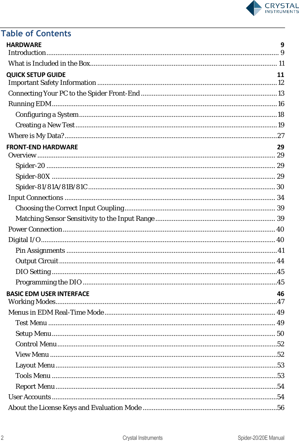
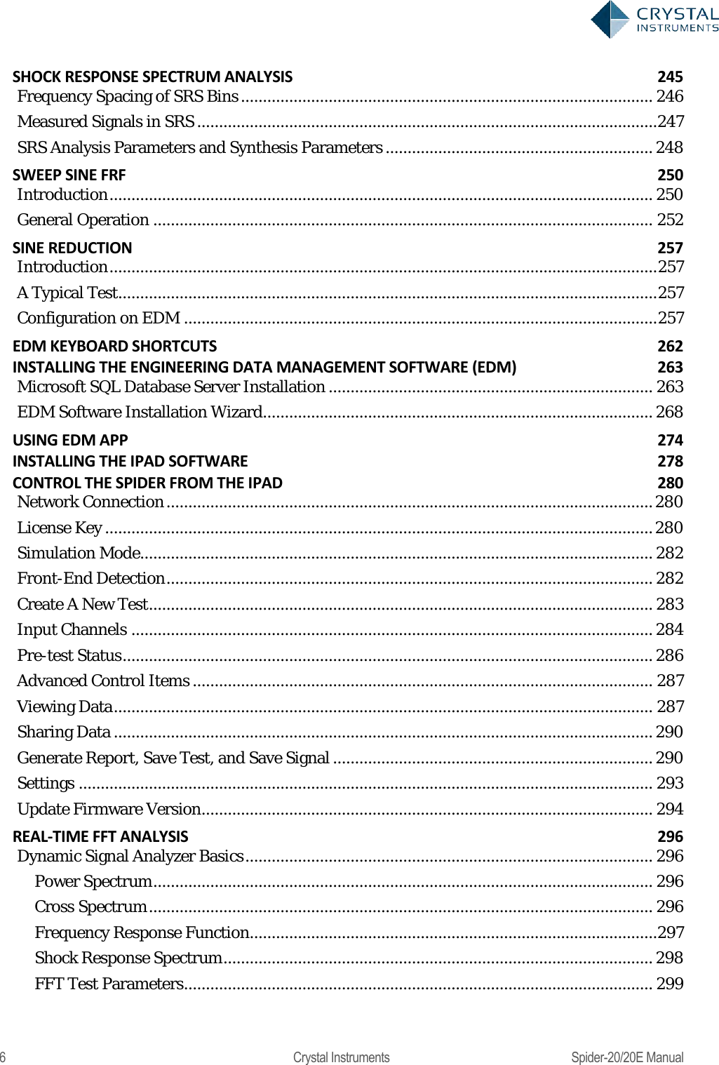

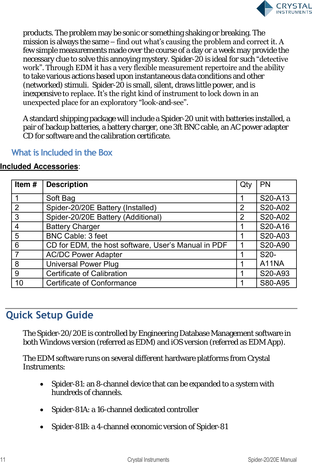
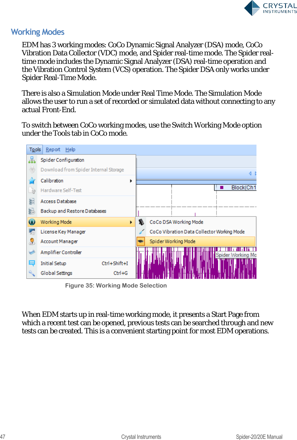
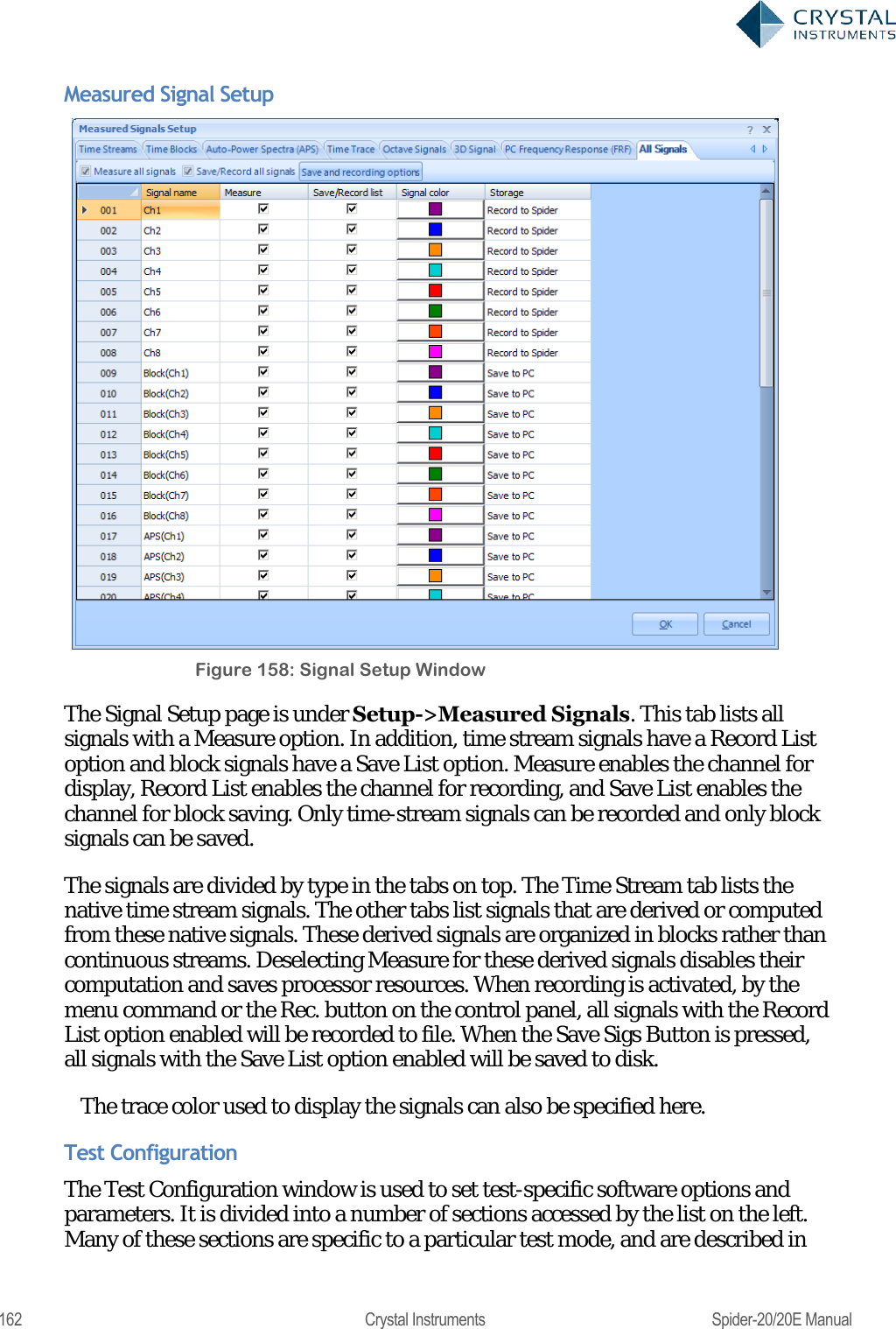
![78 Crystal Instruments Spider-20/20E Manual Figure 75. PC Math Signals Operand 1 Operator Operand 2 Math Signal Unit How to calculate Signal1 Plus Signal2 (The same as signals, APS type. Only signals with the same EU can be calculated) [EURMS^2+EURMS^2] = EURMS^2 Signal1 Minus Signal2 (The same as signals, APS type. Only signals with the same EU can be calculated) Abs(EURMS^2-EURMS^2) = EURMS^2 Signal1 Multiply Signal2 (The same as signals, APS type. Only signals with the same EU can be calculated) [EURMS^2*EURMS^2] = (EURMS^2) Signal1 Divided by Signal2 (N/A. Treat as CPS if both signals are APS.) [EURMS^2*EURMS^2] = N/A Signal Plus Constant (The same as signals, APS type) [EURMS^2 + const^2] Signal Minus Constant (The same as signals, APS type) [EURMS^2 - const ^2] Signal Multiply Constant (The same as signals, APS type) Apply the constant to the original data (EURMS^2) Signal Divided by Constant (The same as signals, APS type) Apply the constant to the original data (EURMS^2) Constant Plus Signal (The same as signals, APS type) [EURMS^2 + const ^2] Constant Minus Signal (The same as signals, APS type) [const ^2-EURMS^2] Constant Multiply Signal (The same as signals, APS type) Apply the constant to the original data (EURMS^2) Constant Divided by Signal (The same as signals, APS type) Apply the constant to the original data (EURMS^2)](https://usermanual.wiki/Crystal-Instruments/SPIDER20.User-Manual-1/User-Guide-3054602-Page-78.png)
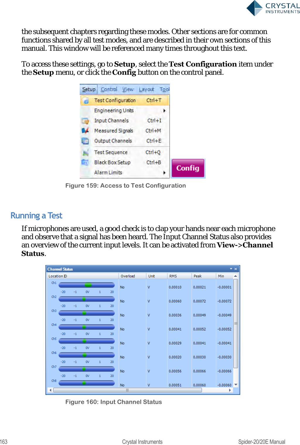
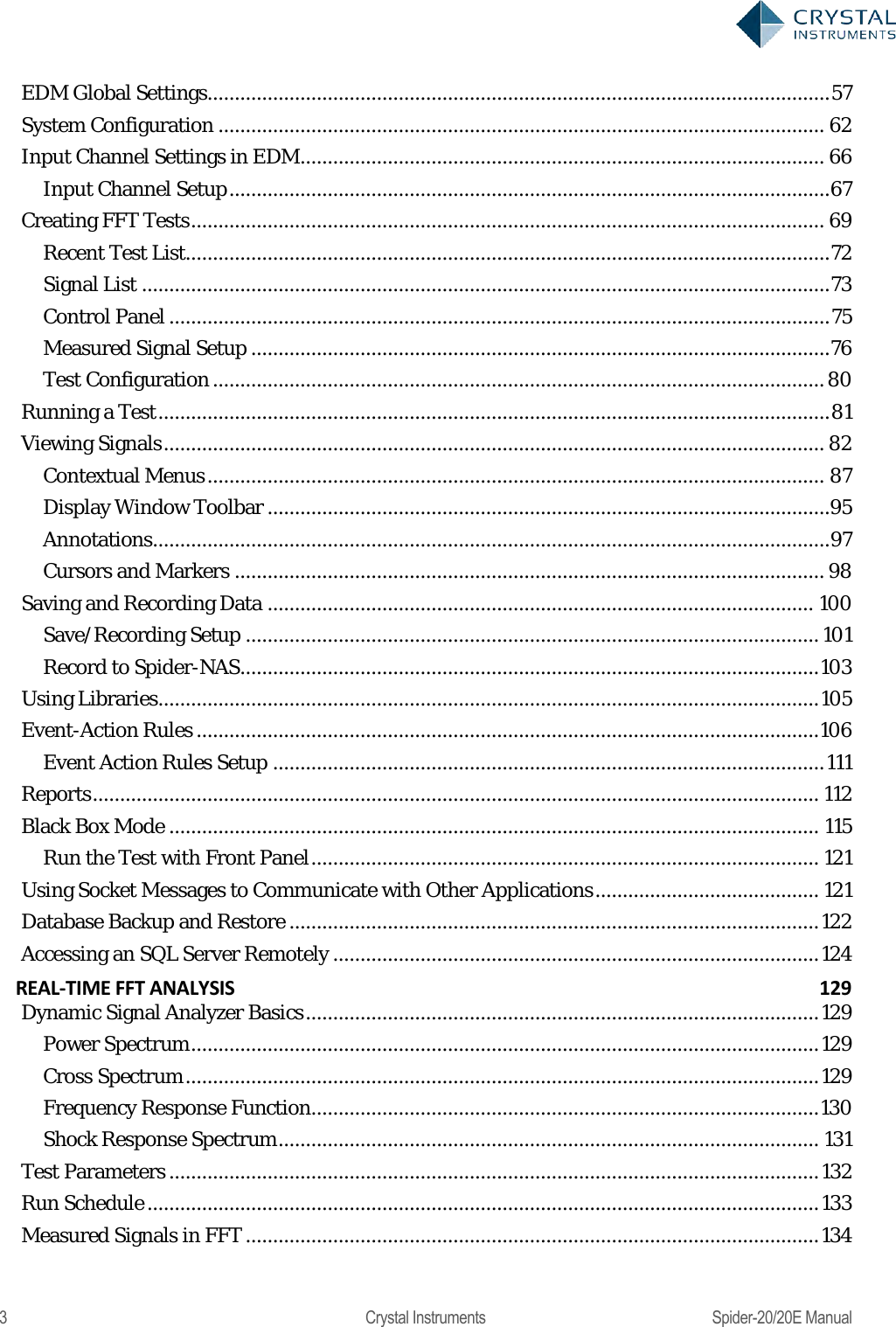
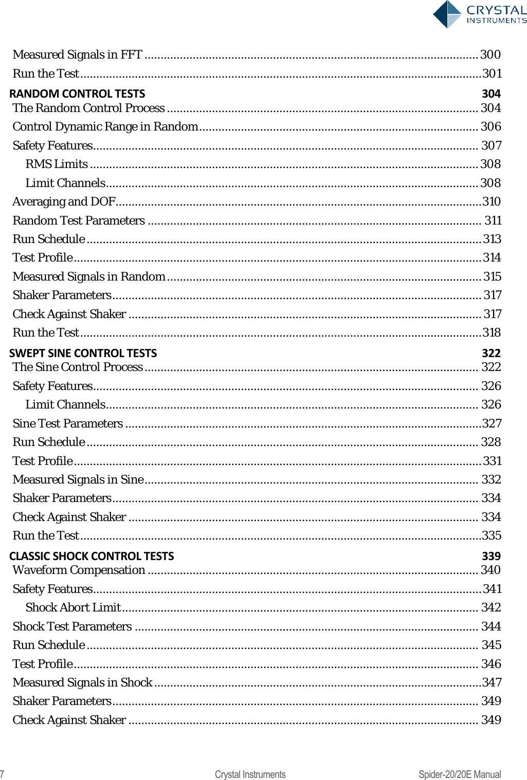
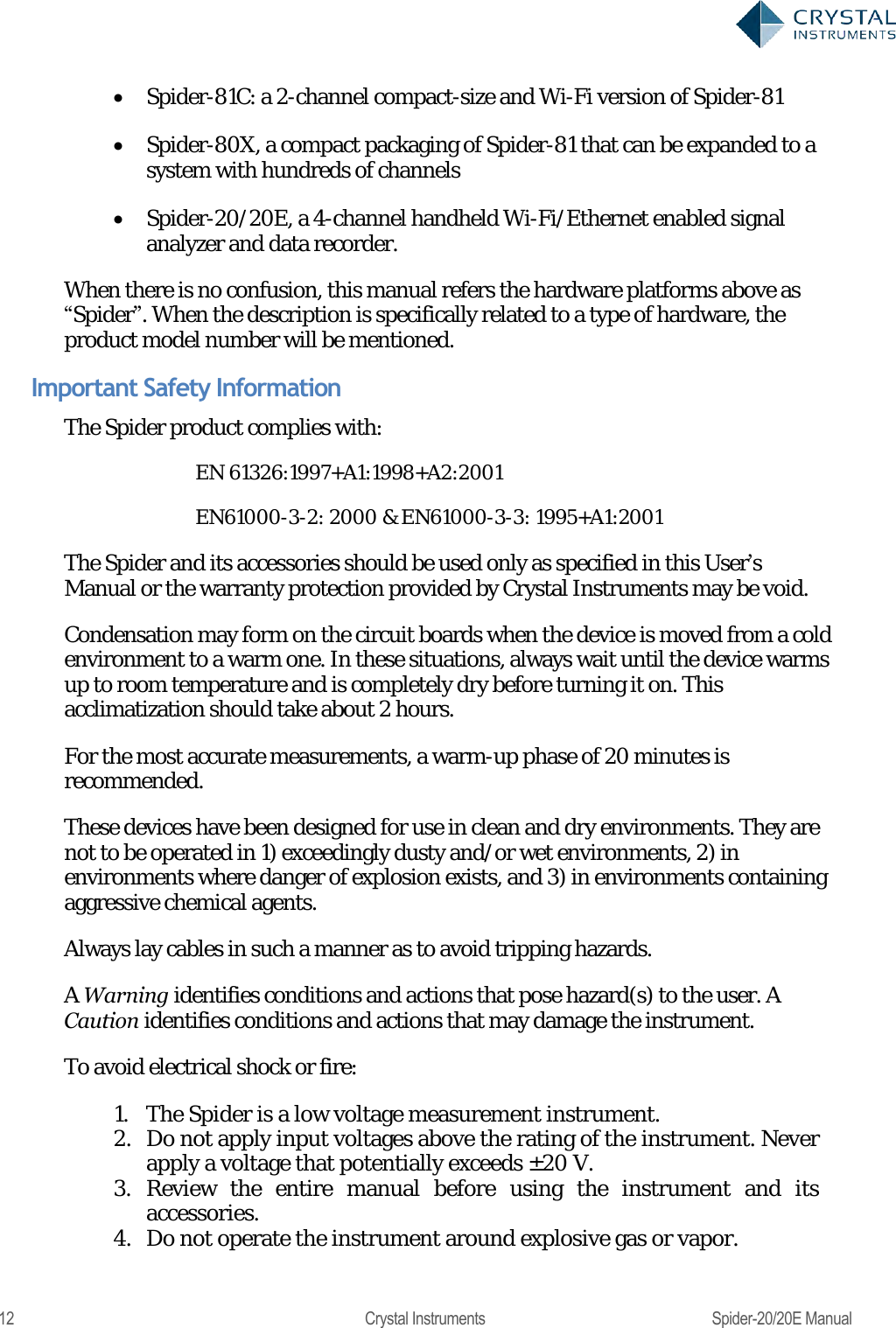
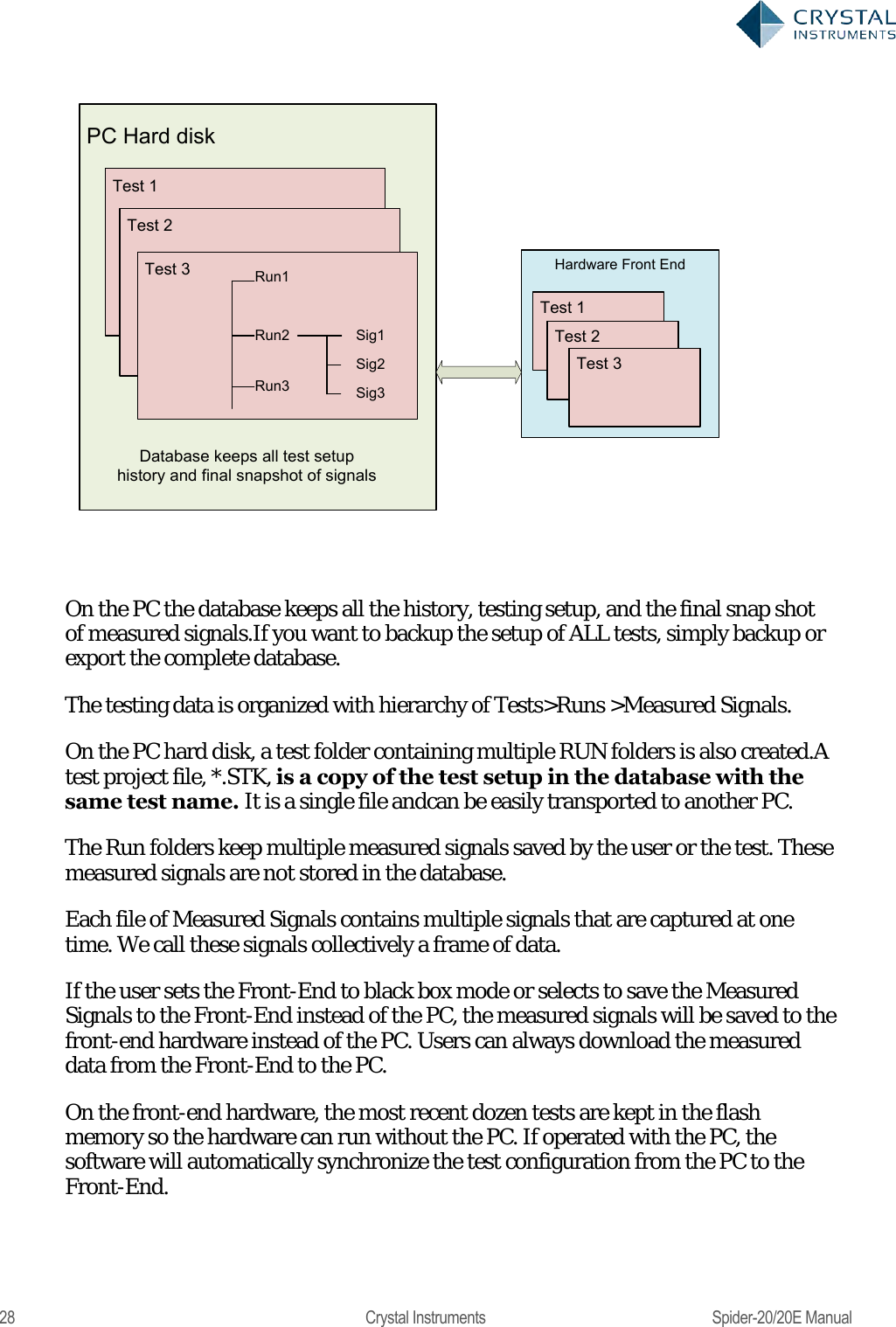
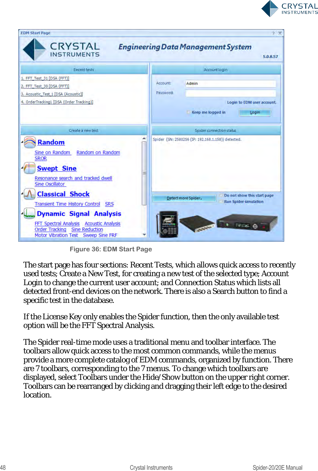
![79 Crystal Instruments Spider-20/20E Manual In the On-board FRF tab (only available when FRF box was checked at the time of creating the test), the Spider calculates the FRF signals and transmits it to the PC for display. Any one channel in the Spider system can be specified as the reference channel by clicking the Change Reference Channel button and selecting the proper channel. Figure 76. On-board FRF Signals In the PC FRF tab, FRF signals are calculated by the PC instead of the Spider. Since the PC FRF relies on the PC‘s resource which is much more powerful than the Spider‘s processor, hundreds of FRF signals can be computed simultaneously without consuming the Spider‘s resource. Multiple channels can be specified as reference channels. The relationship between input (force excitation) and output (vibration response) of a linear system is given by: = where {Y} and {X} are the vectors containing the response spectra and the excitation spectra, respectively, at the different DOFs in the model, and [H] is the matrix containing the FRFs between these DOFs. The equation above can also be written as: =](https://usermanual.wiki/Crystal-Instruments/SPIDER20.User-Manual-1/User-Guide-3054602-Page-79.png)
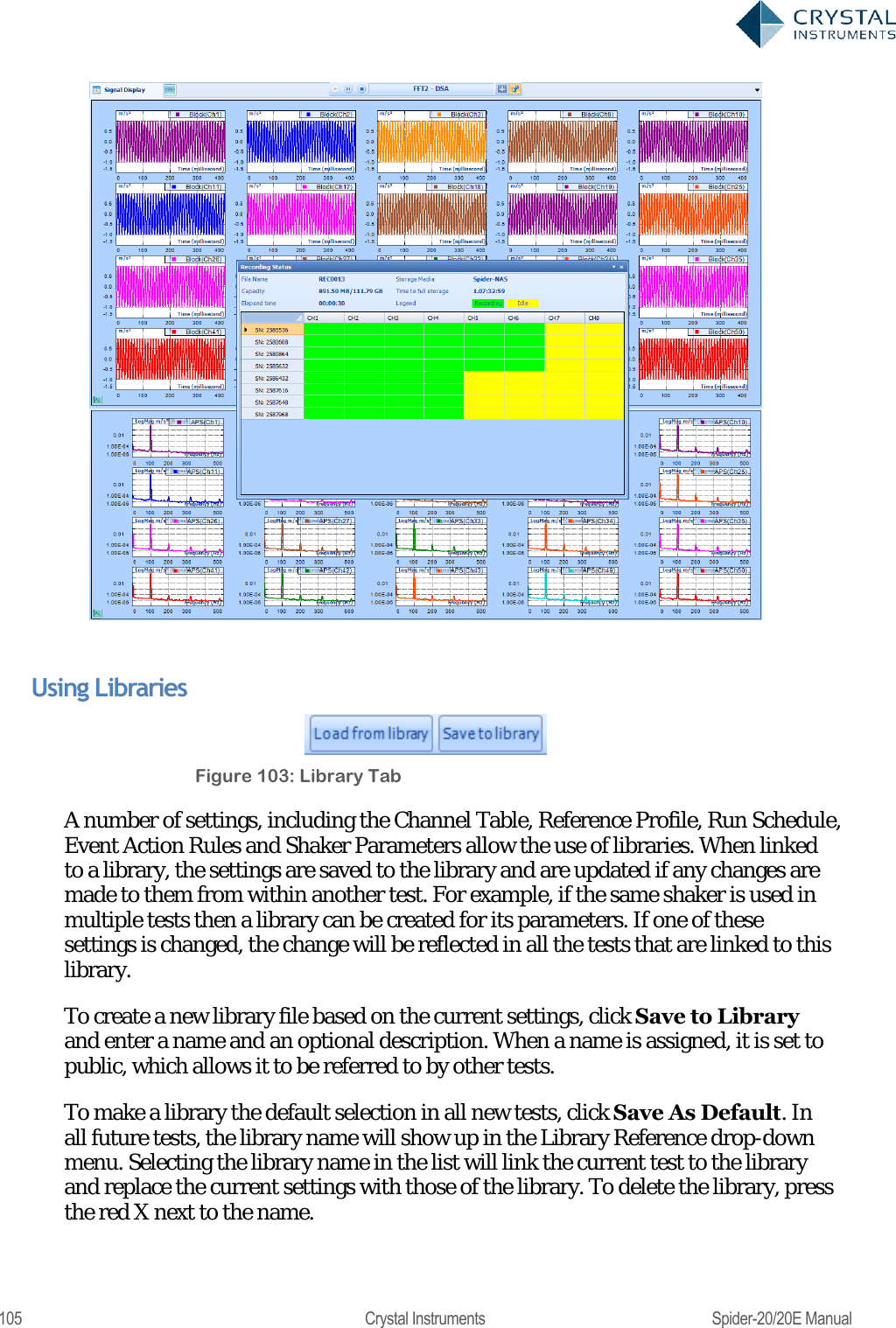
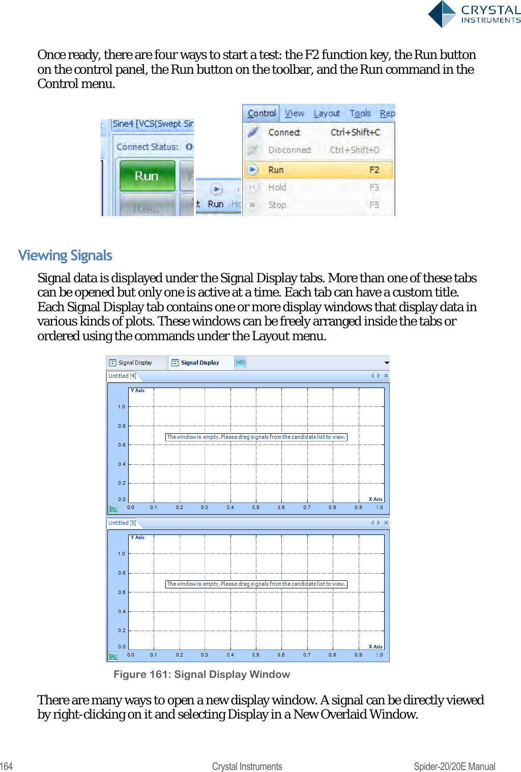
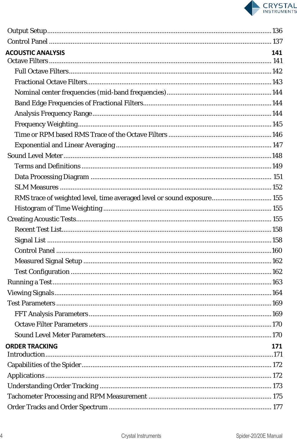
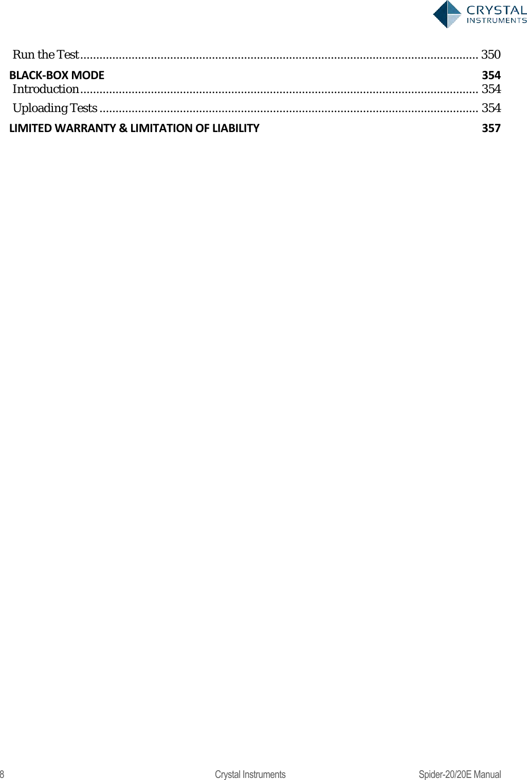
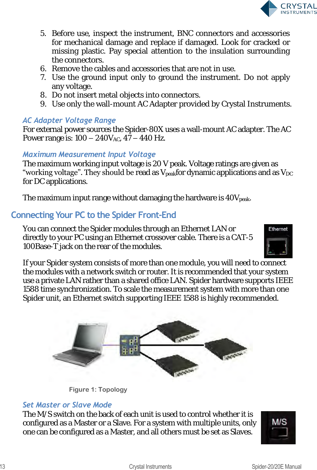
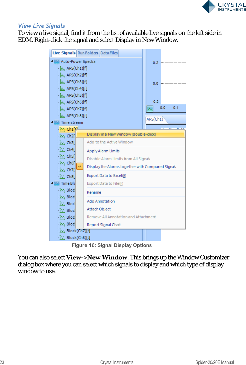
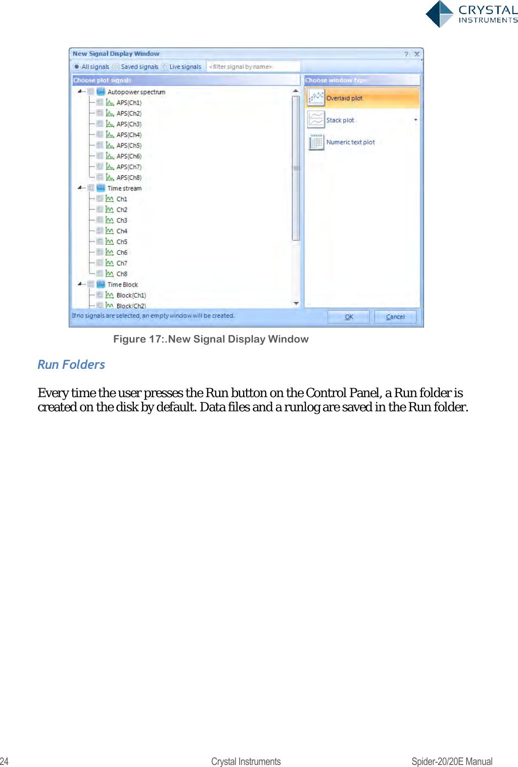
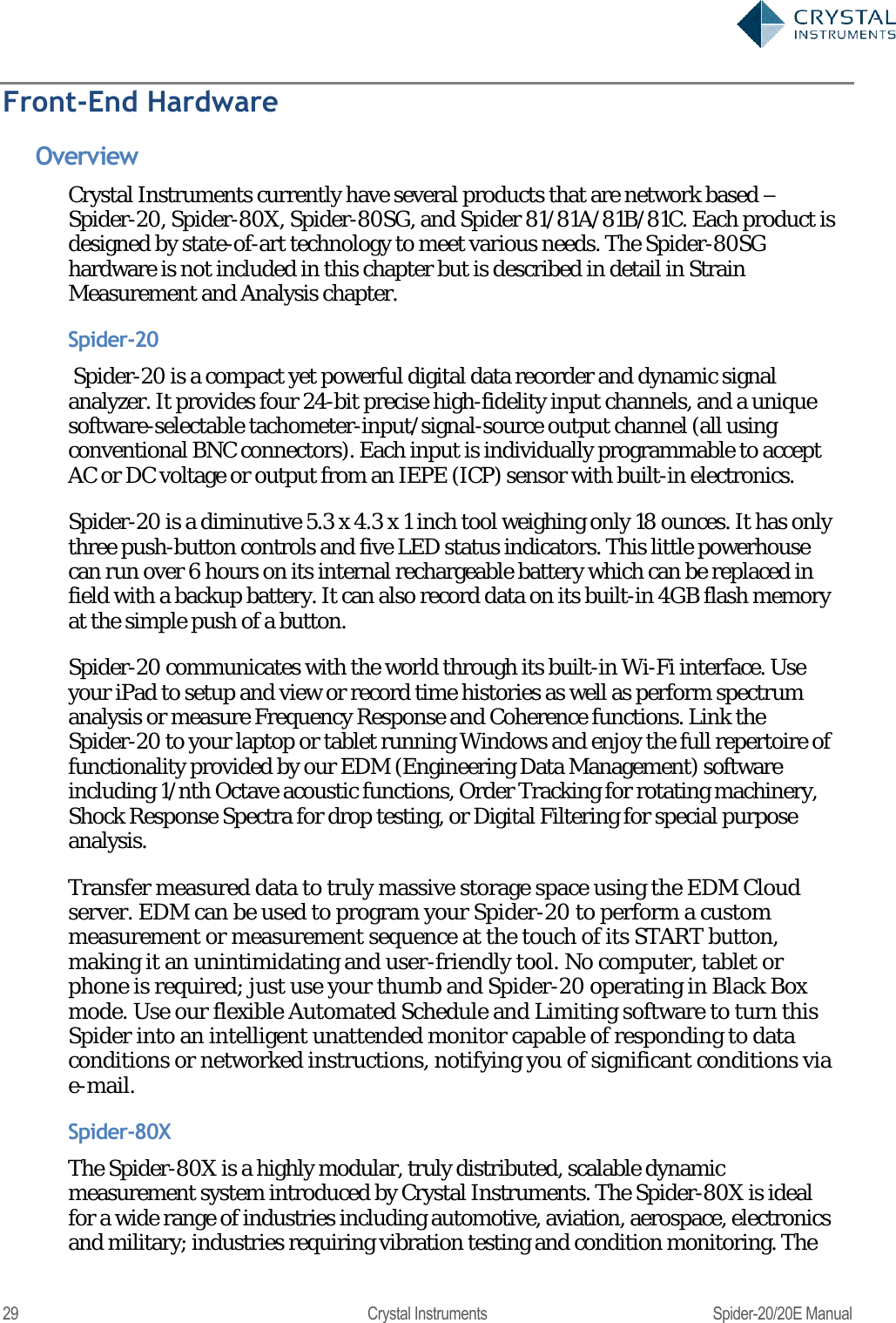
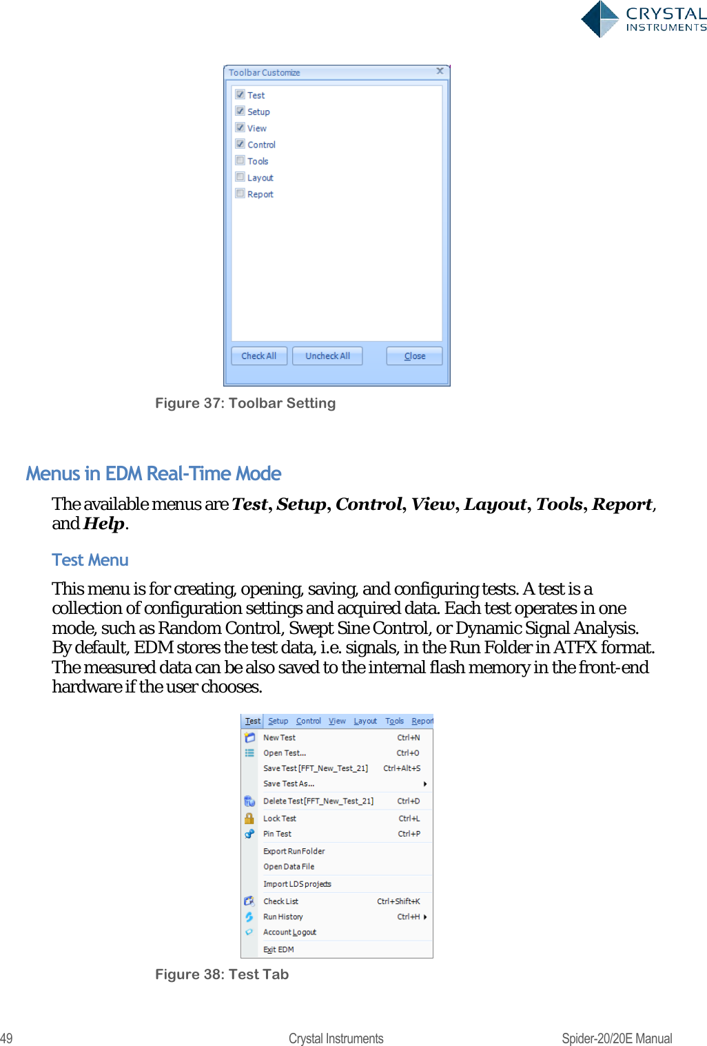
![134 Crystal Instruments Spider-20/20E Manual Figure 131. Run Schedule Tab Measured Signals in FFT The ―Live Signals‖ tab on the lower left of the screen in EDM shows all the measured signals available for display. Listed here, for all test modes, are the time streams of the input channels labeled by their location ID (―PT1‖, ―PT2‖, ―PT3‖… by default), and the output drive time stream. The location ID of the channels can be changed under the Channel Table tab. Time stream signals are labels as Ch1[t]. The numerical value depends on the channel index.](https://usermanual.wiki/Crystal-Instruments/SPIDER20.User-Manual-1/User-Guide-3054602-Page-134.png)
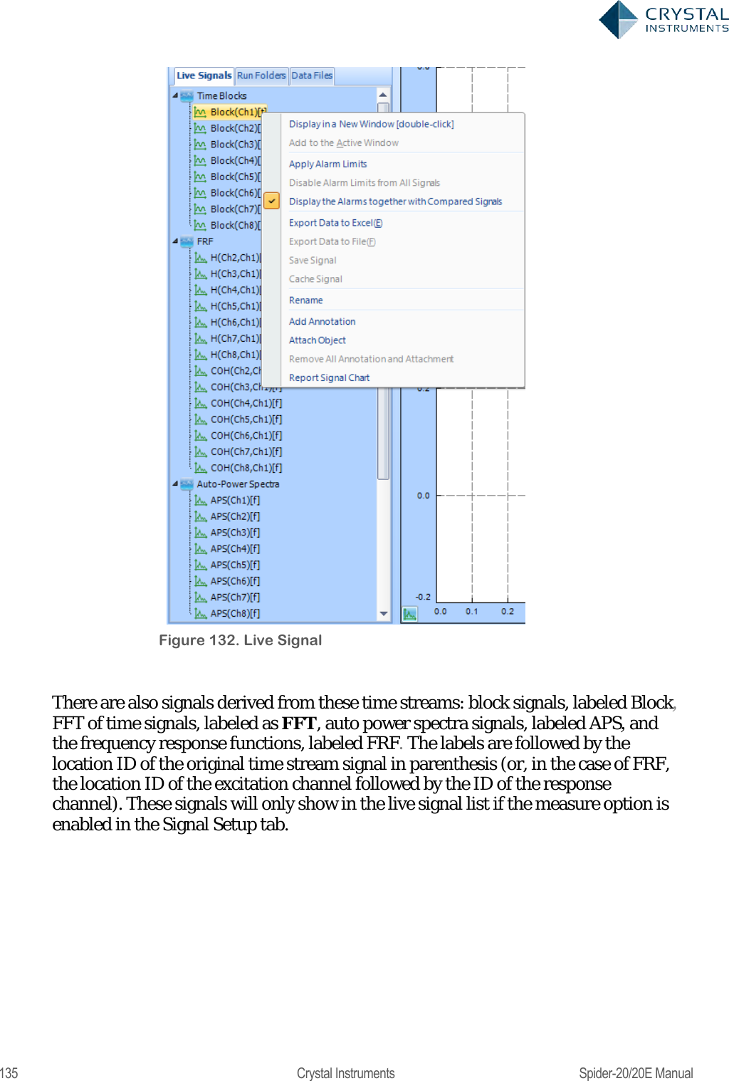
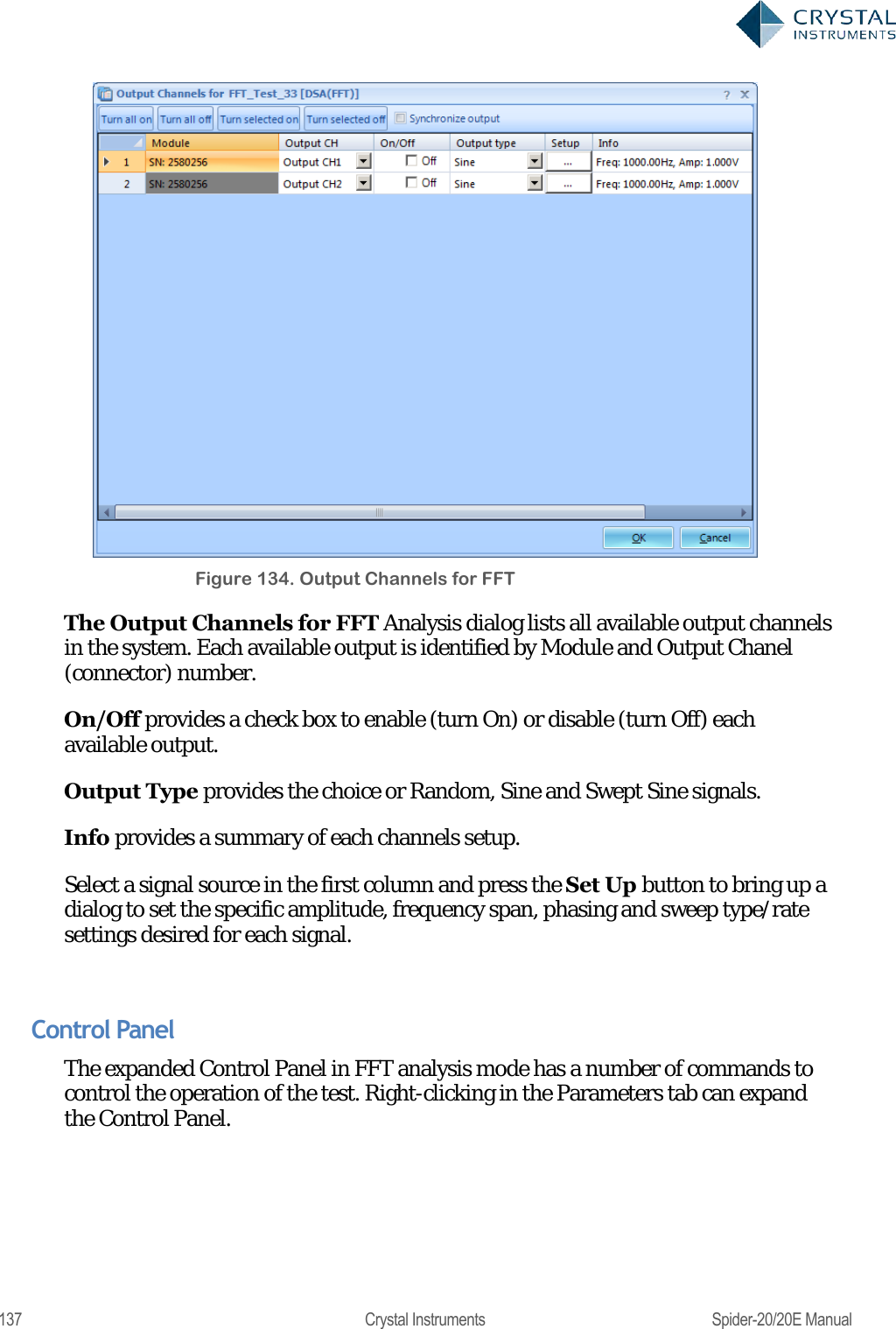
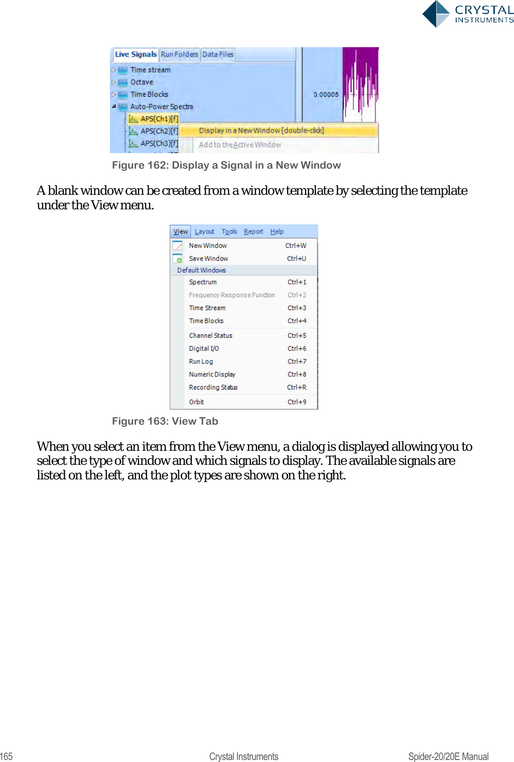
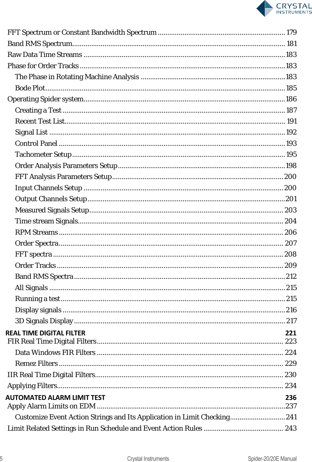
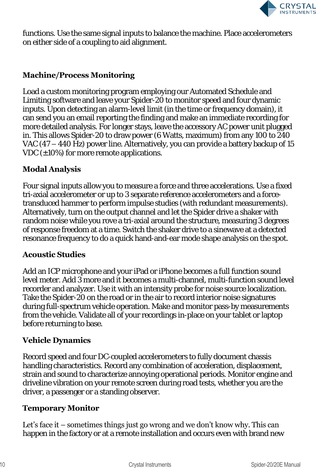
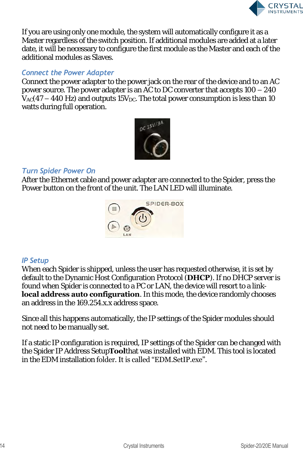
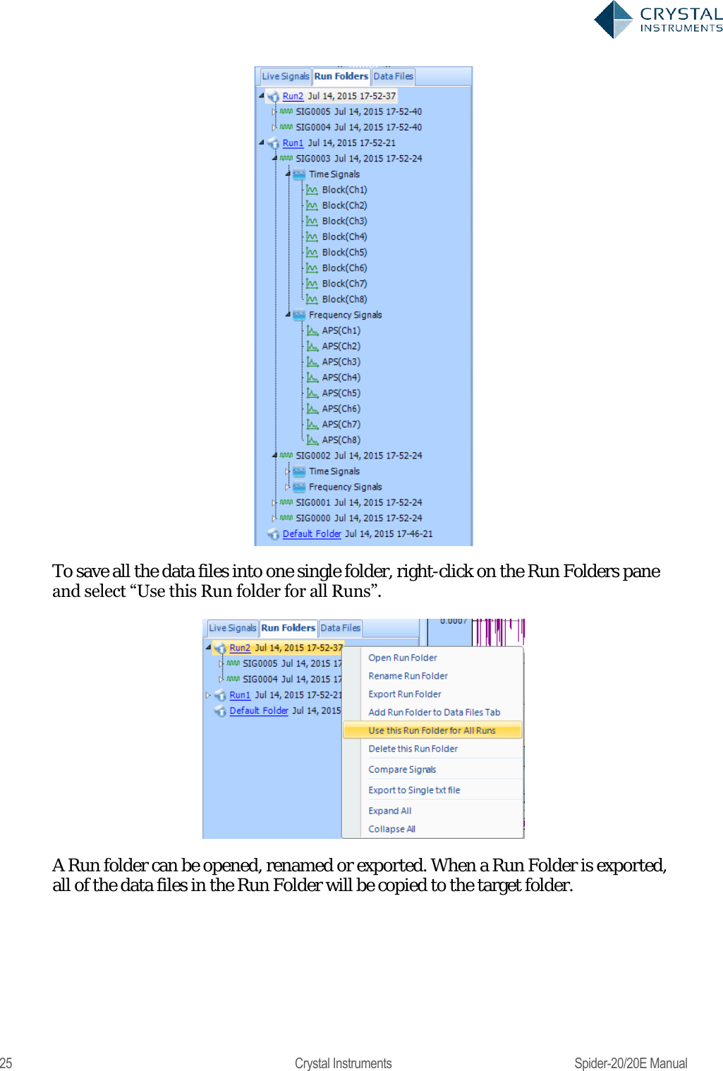
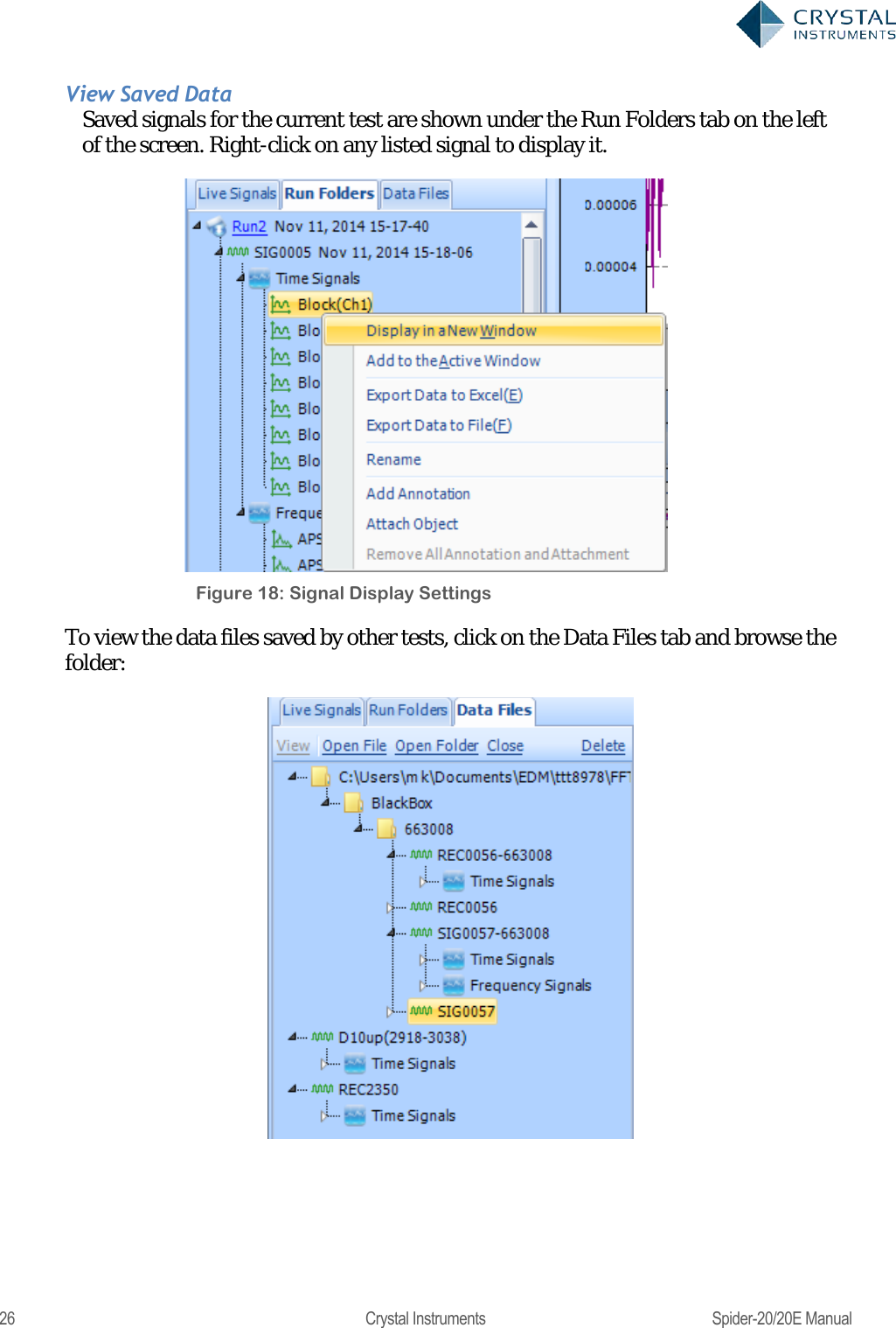
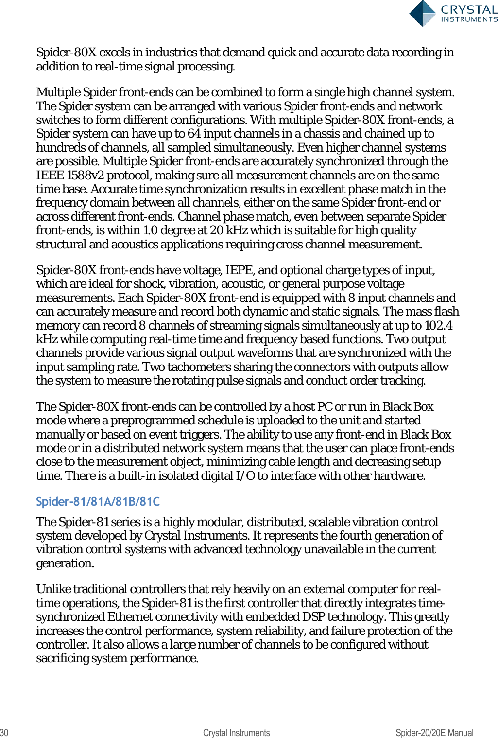
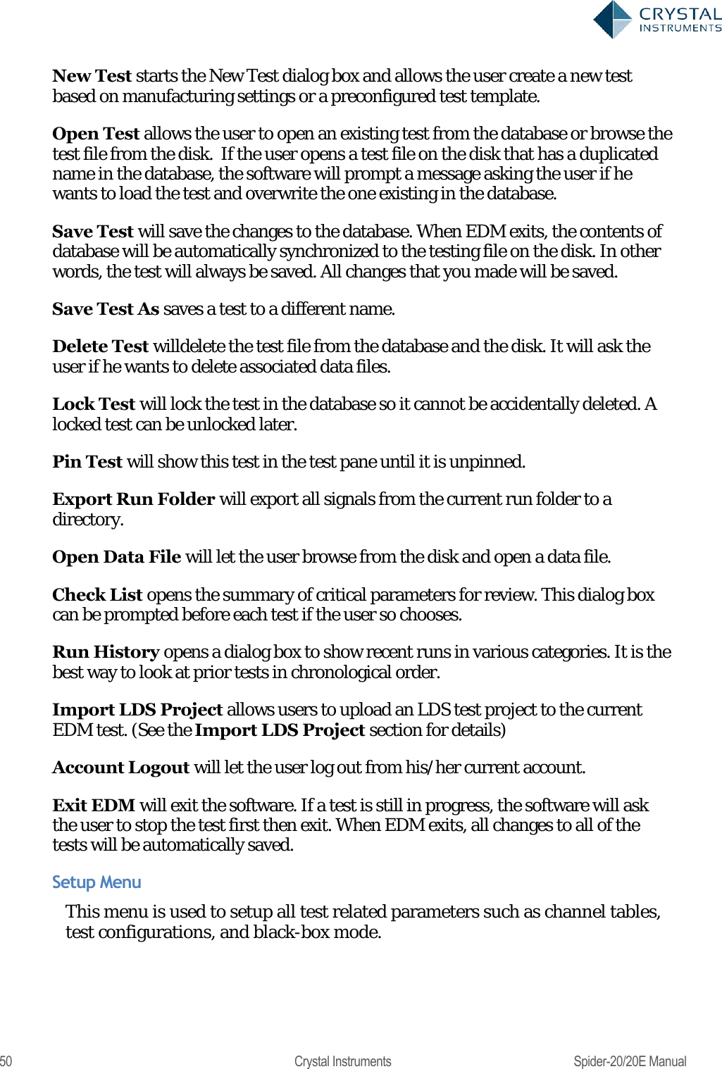
![136 Crystal Instruments Spider-20/20E Manual Figure 133 Frequency response functions measured in a high channel count system Time block signals are labels as Block(Ch1)[t]. The numerical value depends on the channel index. For the convenience of signal calculation and transformation, the time stream is chopped into the individual blocks by block size. Each block contains the defined number of data points sampled from the time stream signals. APS (Auto-Power Spectrum) signals are labeled as APS(Ch1)[f]. The numerical value depends on the channel index. Output Setup The FFT test has an additional tab for output channel setup. Here you can configure one or more output channels as shaker drive or other DUT stimulation signals. Since closed loop control is not available, the user should be careful to stay within the safety limits of the shaker/amplifier and test object when configuring the output levels. All enabled channels will send out drive signals while the test is running. The following window can be found from Setup->Output Channels.](https://usermanual.wiki/Crystal-Instruments/SPIDER20.User-Manual-1/User-Guide-3054602-Page-136.png)