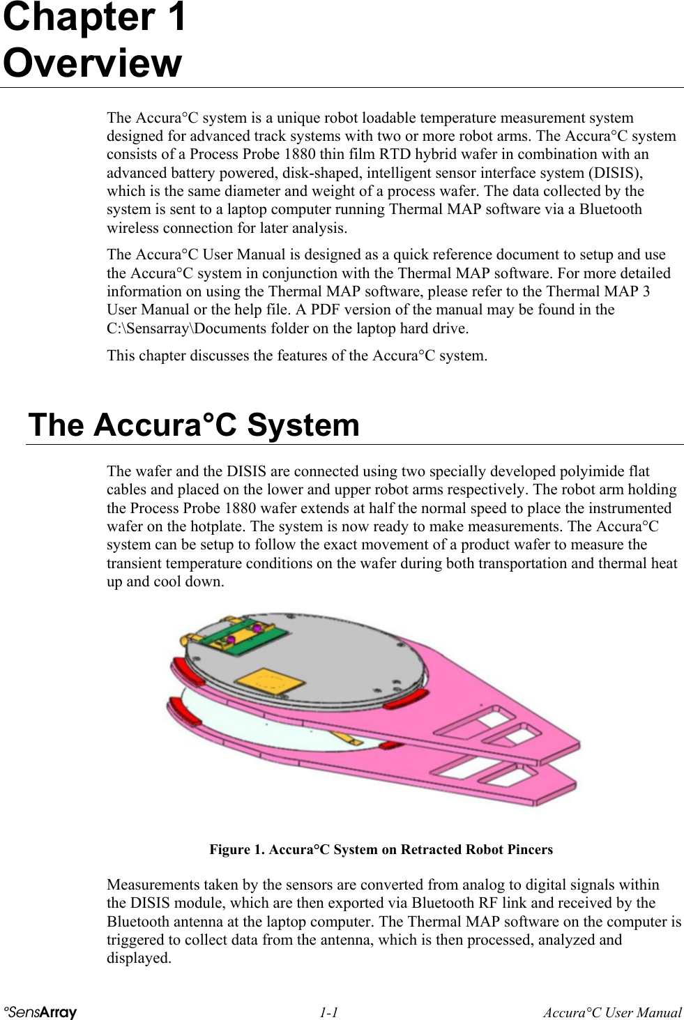
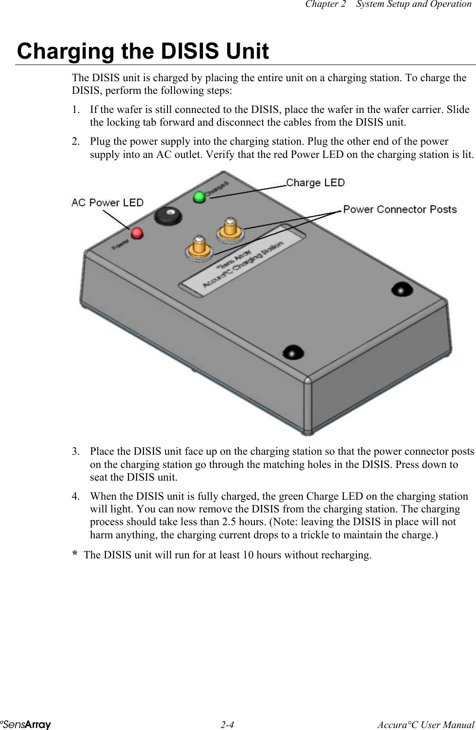
KLA Tencor 482-22-0800 Bluetooth Test and Calibration Device User Manual TMAP 3 Cover

KLA-Tencor Corporation Bluetooth Test and Calibration Device TMAP 3 Cover

Contents

Revised user manual 1 of 2
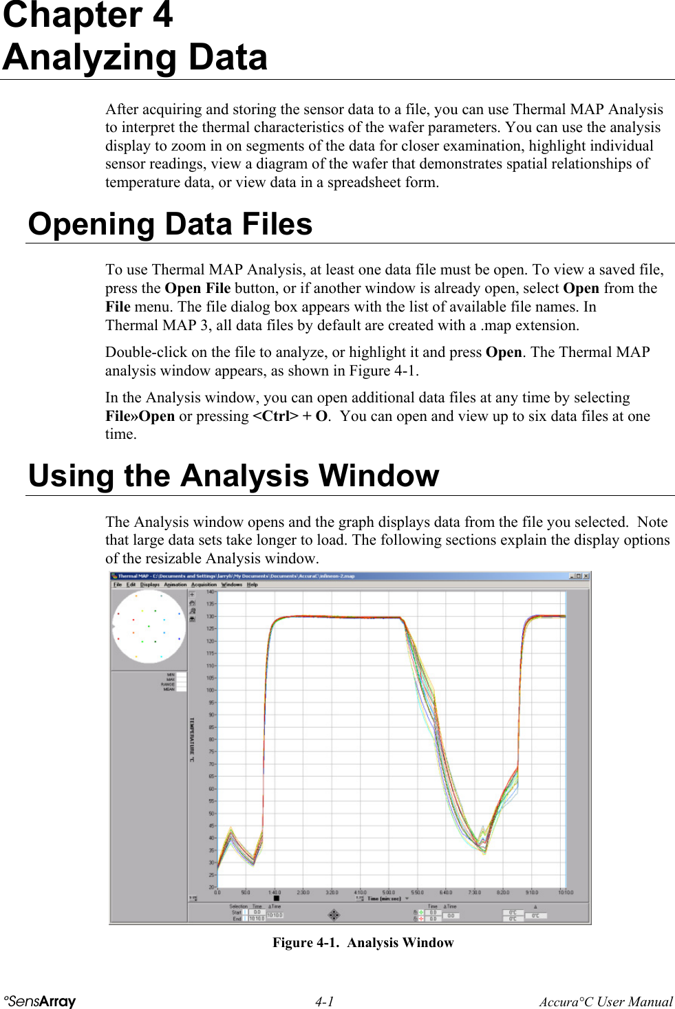
Accura°C User Manual               °SensArray 47451 Fremont Blvd. Fremont, CA 94538  510-360-5600 Fax 510-360-5601 info@sensarray.com www.sensarray.com
 Copyright © 2003 by °SensArray® Corporation. All rights reserved.                              UM-ACC-A 2003.02 This manual applies to the 3.0.6 version of Thermal MAP software.  °SensArray reserves the right to modify, change, or improve any or all specifications published in this document without notice.
Important Notices Warranty Thermal MAP Software SensArray Corporation warrants that (a) Thermal MAP software (Software) will perform substantially in accordance with the accompanying written materials for a period of 12 months after shipment, and (b) the medium on which the Software is recorded will be free from defects in materials and workmanship under normal use and service for a period of 12 months after shipment. Faults caused by unauthorized modification, misuse or abuse of products, or problems due to software not supplied by SensArray, are not covered by this Warranty. During the Warranty Period, the purchaser may return failed Software to SensArray for repair or replacement, at SensArray’s option. SensArray does not warrant that the operation of the Software shall be uninterrupted or error free. The purchaser will first notify SensArray of the nature of the problem and obtain a Returned Materials Authorization [RMA] number. The purchaser will pay the costs of shipping returned Software to SensArray; SensArray will pay the cost of shipping repaired/replaced Software to the purchaser. No other warranty is expressed or implied. SensArray specifically disclaims the implied warranty of merchantability and fitness for a specific application. The Thermal MAP Software Documentation Materials (“Documentation”) are subject to revision and change without notice. SensArray agrees to make a best effort attempt to keep the purchaser advised of changes to the Documentation. Accura°C System Hardware SensArray Corporation warrants that the Accura°C Systems (“Products”) sold will be free from defects in material and workmanship, and perform to SensArray’s applicable published specifications for a period of 12 months after shipment. The liability of SensArray hereunder shall be limited to replacing or repairing, at its option, any defective Products that are returned F.O.B. to SensArray’s plant in Fremont, CA. In no case are Products to be returned without the purchaser first obtaining SensArray’s permission and Returned Materials Authorization [RMA] number. In no event shall SensArray be liable for any consequential or incidental damages. Products that have been subject to abuse, misuse, accident, alteration, neglect, or unauthorized repair or installation are not covered by this warranty. SensArray will make the final determination as to the existence and cause of any alleged defect. SensArray is not responsible for maintaining or supplying any consumable materials used in conjunction with this hardware and SensArray is not liable for expendable items such as fuses, lamps, paper, ink, etc. No warranty is made with respect to any customized equipment or Products supplied with Accura°C systems where produced to Purchaser’s specifications except as specifically stated in writing by SensArray in the contract for such Products. The purchaser will pay the shipping costs of returned materials to SensArray; SensArray will pay the cost of shipping repaired/replaced material to Purchaser. This Warranty is the only warranty made by SensArray with respect to the Product delivered hereunder and may be modified only by a written instrument that is signed by a duly authorized officer of SensArray and accepted by Purchaser. Except as provided above, SensArray makes no warrantees, expressed or implied, including any warranty of merchantability for a particular purpose.
Software License Agreement The Software is owned by SensArray Corporation and is protected by United States copyright laws and international treaty provisions. Therefore, you must treat the Software like any other copyrighted material. Under the Copyright Laws, the Thermal MAP Software, or accompanying written materials, may not be copied, photo-copied, reproduced, translated, in whole or in part, without the prior written permission of SensArray.  You may make one copy of the Software solely for backup or archival purposes. You may make 10 copies of the written materials accompanying the SensArray Corporation-produced Software provided that such copies are solely for use by personnel using Thermal MAP. All rights not expressly granted to you in this Agreement are reserved to SensArray Corporation. Third-Party Software Licenses for any software which was provided but not produced by SensArray Corporation are granted solely and only by the original supplier or manufacturer and solely and only with the supplier’s limitations and rights. Copying restrictions for such software are governed solely and only by the original supplier or manufacturer’s license or any other supplier-approved agreements, as applicable. Trademarks °SensArray®, Thermal MAP®, and Accura°C are trademarks of SensArray Corporation.  Windows and Excel are trademarks or trade names of Microsoft Corporation.  Any other terms mentioned in this document that are known to be trademarks or service marks have been appropriately capitalized. Use of a term in this document should not be regarded as affecting the validity of any trademark or service mark. FCC Compliance Statement:  This device complies with part 15 of the FCC Rules. Operation is subject to the following two conditions: (1) This device may not cause harmful interference, and (2) this device must accept any interference received, including interference that may cause undesired operation. CAUTION: Changes or modifications not expressly approved by the manufacturer responsible for compliance could void the user’s authority to operate the equipment. Important Note: To comply with FCC RF exposure compliance requirements, the antenna used for this transmitter must be installed to provide a separation distance of at least 20cm from al persons and must not be co-located or operating in conjunction with any other antenna or transmitter. European Union Notice   This system has been tested for conformance with CE radio spectral, EMC and safety requirements.
 °SensArray 1-1 Accura°C User Manual Chapter 1 Overview The Accura°C system is a unique robot loadable temperature measurement system designed for advanced track systems with two or more robot arms. The Accura°C system consists of a Process Probe 1880 thin film RTD hybrid wafer in combination with an advanced battery powered, disk-shaped, intelligent sensor interface system (DISIS), which is the same diameter and weight of a process wafer. The data collected by the system is sent to a laptop computer running Thermal MAP software via a Bluetooth wireless connection for later analysis. The Accura°C User Manual is designed as a quick reference document to setup and use the Accura°C system in conjunction with the Thermal MAP software. For more detailed information on using the Thermal MAP software, please refer to the Thermal MAP 3 User Manual or the help file. A PDF version of the manual may be found in the C:\Sensarray\Documents folder on the laptop hard drive. This chapter discusses the features of the Accura°C system.  The Accura°C System The wafer and the DISIS are connected using two specially developed polyimide flat cables and placed on the lower and upper robot arms respectively. The robot arm holding the Process Probe 1880 wafer extends at half the normal speed to place the instrumented wafer on the hotplate. The system is now ready to make measurements. The Accura°C system can be setup to follow the exact movement of a product wafer to measure the transient temperature conditions on the wafer during both transportation and thermal heat up and cool down.  Figure 1. Accura°C System on Retracted Robot Pincers Measurements taken by the sensors are converted from analog to digital signals within the DISIS module, which are then exported via Bluetooth RF link and received by the Bluetooth antenna at the laptop computer. The Thermal MAP software on the computer is triggered to collect data from the antenna, which is then processed, analyzed and displayed.
Chapter 1    Overview Accura°C User Manual  1-2  °SensArray  Acquiring Data The Thermal MAP software acquires and logs the data collected by the Accura°C system. With the Thermal MAP data acquisition features, you can simultaneously view and log wafer temperature sensor data. The data is observed on the strip charts and digital readouts during the acquisition.  The software allows the user to determine how often and for how long the data points will be collected. The user may chose which temperature scale the data will be calculated in, or display the direct resistance output of each sensor on the wafer. Thermal MAP measures the uncorrected sensor signals, applies corrections for sensor and data acquisition system calibration offsets, then converts the readings to temperature. The data is saved to the laptop hard disk for later analysis. Analyzing Data Previously logged data files may be analyzed using a powerful graphic interface to view XY graphs, contour maps, surface maps, animations, and data tables. The logged data is stored in a data table. Thermal MAP Analysis graphics can be viewed directly without opening the data table. Or the data can be viewed and evaluated in table form, if desired.  A row in the table is called a sample or a single-timed sampling of all of the sensors on the wafer and system inputs. You use the sample number to identify the table row of measurements collected at the sample time. The first column in the table is the sample number. The second column is the elapsed time at which the sample was acquired. For example, as shown in Figure 2, Sample# 0 has a time of zero. The remaining columns in the table are the temperatures of the individual RTD sensors within the wafer. Additional columns of data can be present if system sensors, digital, and/or calculated values have been logged. In addition to the data within the table, the data file stores other pertinent information—including run date and time, operator’s name, and a description of the test—which you enter before acquisition.
   Chapter 1    Overview °SensArray 1-3 Accura°C User Manual  Figure 2.  Sample Data Table During acquisition, Thermal MAP performs computations on acquired data, such as determining the minimum, maximum, mean, range (max-min), and standard deviation of all wafer sensor values for the sample, and logs the results in columns. These computed values are referred to as calculated values. After acquiring, linearizing, and storing the sensor data, you can display or print the data as a line plot graph, as shown in Figure 3. In addition, you can display data in a table or as a wafer map.  Figure 3.  Displaying Data on a Line Plot Graph
Chapter 1    Overview Accura°C User Manual  1-4  °SensArray  You can also display a 2-dimensional color contour map as shown in Figure 4 or a 3-dimensional surface map as shown in Figure 5.   Figure 4.  Two-Dimensional Color Contour Map  Figure 5.  Three-Dimensional Surface Map With the Animation feature, an animation of the acquired data can be created. The animation can be set for a particular range of the acquired data, saved to a standard AVI file, and replayed at any time. The AVI file can be sent to other computers not running the Thermal MAP software and played using the Windows Media Player With the Derived Files Feature, statistical data can be generated for selected periods of an acquisition run. In addition, the differences in selected sensor readings between two different acquisition runs may be compared. Data may also be exported to a spreadsheet program, edited in the spreadsheet, and loaded back to Thermal MAP for further analysis.
 °SensArray 2-1 Accura°C User Manual Chapter 2 System Setup and Operation Before you can begin working with the Accura°C system, you need to unpack the system components, prepare the equipment for transfer to the cleanroom, and connect the system cables. Connecting the System Before shipping, SensArray assembles and tests the Accura°C system. The Thermal MAP software is preinstalled and configured. To setup the system, you only need to connect the cable from the wafer to the DISIS unit and install the Bluetooth module to the laptop.   Do not load any additional software on the system hard drive. All required software is loaded and tested prior to shipping. Connecting the Wafer to the DISIS To connect wafer and DISIS unit, complete the following instructions. 1.  Slide the locking tab on the wafer connector forward to unlock the connector.   Figure 1. Connector Board Components 2.  Place the DISIS unit and the wafer so that the twin cable and connector face each other as shown in Figure 2.
  Chapter 2    System Setup and Operation °SensArray 2-2 Accura°C User Manual  Figure 2. Wafer DISIS Connection 3.  Place the wafer connector over the guide pins of the DISIS connector and press down to firmly seat the connector. Slide the locking tab back to lock the connection.  Turning the System On After all the component connections are completed, the system is turned on to verify proper operation.  1.  Locate the power switch on the laptop and turn the power ON. If the system turns on successfully, Windows 2000 logon screen will appear.  2.  Logon to Windows 2000. The system is shipped with the password field blank (no password) and you only have to hit <Enter> to log on to the system.  3.  Plug the Bluetooth adapter into a USB port.  4.  Verify that the DISIS unit is turned on. The green LED next to the connector should be flashing. If not, press and hold the Power button on the DISIS for at least one second. (To turn the power off, just press the power button a second time.)  Figure 3. DISIS Component Locations 5. Open My Bluetooth Places from the desktop.
  Chapter 2    System Setup and Operation °SensArray 2-3 Accura°C User Manual 6. Open Entire Bluetooth Neighborhood and read the list of Bluetooth items available. If there is more than one DISIS unit assigned to the system, locate the DISIS with the same serial number as the DISIS unit you are using for the test. Double-click on the ISIS unit icon.  7.  Check that the serial port shows Connected. If not, right-click on the icon and select Connect Serial Port. Note the number of the COM port displayed in the right-hand column. 8.  Launch the Thermal MAP Software by clicking on the Thermal MAP icon on the desktop. 9. Click on Acquisition. If the DISIS is not found, click on Select Serial Port and set the serial port to the number noted above. Then click Retry. 10.  Once the DISIS unit is recognized, acquire data normally.  Loading the System on the Robot Arms To place the system on the robot arms, complete the following instructions. 1.  Have the operator extend the bottom robot arm. The robot should be moving at no more than 50% speed. 2.  Carefully remove the wafer from the wafer carrier with one hand. With the other hand, pick up the DISIS unit. Keep the DISIS unit above the wafer. 3.  Carefully place the wafer on the lower robot arm. 4.  Keep the DISIS unit clear of the robot extension area and have the operator extend the upper robot arm. Place the DISIS unit on the upper arm.  5.  Align the wafer and DISIS unit so that the two cables are parallel with the robot extension. 6.  Have the operator retract both robot arms.
  Chapter 2    System Setup and Operation °SensArray 2-4 Accura°C User Manual Charging the DISIS Unit The DISIS unit is charged by placing the entire unit on a charging station. To charge the DISIS, perform the following steps: 1.  If the wafer is still connected to the DISIS, place the wafer in the wafer carrier. Slide the locking tab forward and disconnect the cables from the DISIS unit. 2.  Plug the power supply into the charging station. Plug the other end of the power supply into an AC outlet. Verify that the red Power LED on the charging station is lit.  3.  Place the DISIS unit face up on the charging station so that the power connector posts on the charging station go through the matching holes in the DISIS. Press down to seat the DISIS unit. 4.  When the DISIS unit is fully charged, the green Charge LED on the charging station will light. You can now remove the DISIS from the charging station. The charging process should take less than 2.5 hours. (Note: leaving the DISIS in place will not harm anything, the charging current drops to a trickle to maintain the charge.) *  The DISIS unit will run for at least 10 hours without recharging.
Chapter 3 Acquiring Data This chapter discusses Thermal MAP® 3 Acquisition, including a thorough explanation of the following areas. •  Acquisition Setup—Setting acquisition options  •  Additional Acquisition Features—Configuring hardware and calculated channels, and setting triggers •  Acquisition Display—Setting channel attributes and viewing wafer configurations Acquisition Setup Before acquiring data, you need to set options for the data acquisition run. After starting a run, you can use a graphical stripchart display to view data as it is acquired.  This section discusses operating the configuration editors and setting up the system input and calculated channel configuration files. These files store information on how to acquire and log data for a particular hardware configuration.  In addition, this chapter discusses the following topics.  •  Using Acquisition Setup window options •  Configuring system input and calculated channels for specific process systems, chamber modules and test parameters •  Starting data acquisition Using the Acquisition Setup Window You can begin acquisition by choosing Acquisition when you log onto Thermal MAP 3.  If you are analyzing a previously recorded file, you can begin acquisition by choosing Acquisition»Acquire from the menu bar. If the system is unable to initialize the serial port, please refer to the Thermal MAP 3 User Manual or the help file for troubleshooting information. A PDF version of the manual may be found in the C:\Sensarray\Documents folder on the laptop hard drive. If all the connections are correct, a message briefly appears identifying the DISIS unit and then the Acquisition window shown in Figure 3-1 opens. °SensArray  3-1  Accura°C User Manual
   Chapter 3    Acquiring Data °SensArray  3-2  Accura°C User Manual   Figure 3-1.  Basic Acquisition Setup Window The following table describes fields on the Acquisition Setup window. Field  Description or Result  Operator’s or equipment logon name. The name of the user or equipment from the logon is the default name in the box. The name can be changed by highlighting the current operator name and typing a new name in the box.  This field allows you to enter information regarding the test. You can use the scroll bar to access any information that overflows the window. Update automatically from the system calendar and clock. When the Setup ISIS Wait For Trigger button is pressed, the date and time displays freeze and become the start of acquisition date and time recorded with the data.  Name of the file that logs data. The field defaults to the filename for the previous acquisition. The default data directory is C:\Sensarray\Data. The default file type is .MAP. To change the name of a new file, highlight the current file name and enter a new name. You can leave the Data File field blank and acquire data without writing the data to a file. When you start the acquisition, a prompt confirms that you do not wish to log data. To clear the Data File field, highlight the text and use the <Delete> key to remove the name. To change location of the data file, click on the Browse button to open the Save As dialog box. If you do not want to overwrite an existing file, assign a unique name to the file in the File name field on the Save As dialog box.
   Chapter 3    Acquiring Data °SensArray  3-3  Accura°C User Manual  Field  Description or Result  This specifies the time interval between samples. To set the units, click on the units field and use the popup menu.  To change the resolution for sec (seconds) or min (minutes), you must type in a value. The equivalent rate in Hertz is shown on the right. Alternatively, you can specify a rate in Hertz and the closest sample interval is selected automatically.   Specifies the time period to acquire samples. Dividing the period by the scan interval gives the total number of sets of samples. This number is only an upper limit—you can stop the acquisition manually at any time before the limit is reached.  Note:  After you trigger the acquisition, you cannot modify the Acquire For field.  Figure 3-2.  Sample Rate Controls The controls shown in Figure 3-2, perform the following functions: •  Use the left control to specify the length of time for acquisitions. This value must be higher than Scan Every period. If you put in a value that is lower, the software will automatically adjust the Acquire For period to equal one sample. •  Use the center control to specify the unit. Select seconds, minutes or hours from the popup menu. •  The indicator on the right of the = (equal sign) shows the total number of samples of the acquisition unless stopped prematurely. The indicator updates automatically if you change the Acquire For or Scan Every period. Alternatively, you can enter the number of samples into this field and the time values in the Acquire For period update accordingly.  Specifies the unit of measure for the logged data. When you click on Scale, a popup menu appears. From this menu, select the temperature scale you wish to use:  For RTD-instrumented wafers, you can also select resistance. By selecting resistance, Thermal MAP logs sensor resistance without converting the readings to temperature.
   Chapter 3    Acquiring Data °SensArray  3-4  Accura°C User Manual  Field  Description or Result  Displays the type and serial number of the wafer that will be used. If the system detects the correct wafer, it displays the wafer number in the window. If the correct wafer is not displayed, ensure the calibration file included with your wafer was installed. Select Auto from the popup menu to detect automatically the installed wafer (default). Or you can select other installed wafer configurations from the popup menu. For the Auto command to function properly, a wafer with an ID chip in its connector must be connected to the ISIS unit. From the popup menu, you can access all valid wafer configurations that are currently stored in the Configs folder. However, selecting an incorrect wafer yields invalid readings, graphs and maps.  A message that displays the current status of acquisition, such as Acquisition Setup, Waiting For Trigger, or Acquiring Data.   Once acquisition has begun, this indicator displays the total number of samples that are currently acquired, as well as the total number that the acquisition run will acquire before completion.  Once acquisition has begun, these indicators show the time remaining and the time elapsed.    Using Acquisition Setup Buttons  You can use the following buttons on the bottom of the Acquisition Setup window. Button Description Expands the window to include options for hardware and calculated channel configuration. In addition, you can setup triggering. See the  Additional Acquisition Features section of this chapter for more information. Multi-purpose button used to start or trigger an acquisition, depending on current state. When you complete the acquisition setup, you must press this button to configure the ISIS. Acquisition does not start until the trigger condition is met. If set for manual trigger, this button must be pressed again. Multi-purpose button used to stop an acquisition, or exit the acquisition module, depending on current state.
   Chapter 3    Acquiring Data °SensArray  3-5  Accura°C User Manual  Additional Acquisition Features  With the additional acquisition features, you can define hardware, calculated channel configurations, and set triggering. Press the More Options» button to expand the Acquisition Setup window and open the right-hand pane, as shown in Figure 3-3.   Figure 3-3.  Expanded Acquisition Setup Window For detailed information on using the additional acquisition features, such as hardware configurations or setting system and module information, please refer to the Thermal MAP 3 User Manual located in the C:\SensArray\Documentation folder on your hard disk or use the help file. Setting Calculated Channel Configurations  With Thermal MAP, you can perform computations on the wafer or substrate sensor data and log the results as separate data columns. The Calculated Configuration field on the expanded portion of the Acquisition Setup window displays the configuration selected for the next acquisition. You can select a different configuration from the pull-down menu, as shown below.  If you select New Configuration from the menu, the Calculated Configuration Editor opens. See the next section, Creating and Modifying Calculated Configurations, for more information.  To edit the selected configuration, press the Edit button to open Calculated Configuration Editor. See the next section, Creating and Modifying Calculated Configurations, for more information.
   Chapter 3    Acquiring Data °SensArray  3-6  Accura°C User Manual  Creating and Modifying Calculated Configurations By selecting the New Configuration option or pressing the Edit button under the Calculated Configuration field, you open the Calculated Configuration Editor, as shown in Figure 3-4. With the editor, you have the option of logging specific calculations. The calculations are performed on a sample-by-sample basis. The calculated data is logged for each set of readings at a given time.  Figure 3-4.  Calculated Configuration Editor The following table describes fields, checkboxes, and buttons on the Calculated Configuration Editor window. Fields/Buttons/ Checkboxes  Definition or Result  Includes the minimum sensor reading in the list of calculated channels.  Includes the maximum sensor reading in the list of calculated channels.  Includes the range (maximum–minimum) of the sensor readings in the list of calculated channels.  Includes the arithmetic mean (or average) of the sensor readings in the list of calculated channels.  Includes the standard deviation of the sensor readings in the list of calculated channels.  Includes the wafer rotation position displayed on the Acquisition Display window in the list of calculated channels.  Name you assign to the configuration that you are creating or editing. A new name may be entered or the existing name changed by clicking in the text box and editing or entering the desired name.   Description of the hardware configuration. For example, Standard Wafer Calculated Configuration.  Saves modifications to the configuration.
   Chapter 3    Acquiring Data °SensArray  3-7  Accura°C User Manual  Fields/Buttons/ Checkboxes  Definition or Result  You use this option to save a new configuration for the first time. If the configuration name exists, press this button to create a duplicate configuration of the same name. If you save a duplicate copy, the original version remains displayed. You can view duplicate configurations from the pop-up menu of the Hardware Configuration field on the expanded Acquisition Setup window. The configurations appear in the order of creation.  Opens the help file for this window.  Deletes the currently displayed configuration. The default configuration loads after a deletion.  Cancels any changes you made to a configuration and ends the editing session.  Acquisition Display From strip charts and diagrams on the Acquisition Display window, you can observe data as it is acquired. This section discusses using the Acquisition Display window, setting channel attributes, and viewing wafer or substrate configurations. If a filename was specified in the Acquisition Setup, the Line Plot Display window from the Analysis program will automatically display after acquisition is complete and you exit Acquisition Setup. To display a strip chart as the acquisition is occurring, select Displays»Stripchart Display (or press <Ctrl>+<F5>) from the Acquisition Setup window to open the Acquisition Display window as shown Figure 3-5.  Figure 3-5.  Acquisition Display Window The following table describes the features of the window that you can manipulate to control the display of data.
   Chapter 3    Acquiring Data °SensArray  3-8  Accura°C User Manual  Item Description Strip Chart Displays On the left portion of the window are two strip-charts that display readings and calculated data during acquisition. The upper chart displays readings in units of temperature. The lower chart displays values in units other than temperature. If the display range obscures the plots, you can change the range of the temperature scales to the right by editing the text in the top or bottom label of each scale.   From the popup menu, you can set the number of samples (from 10 to 2000) displayed at one time in the chart.   Changes the background color of the strip chart and map display. The button toggles between a white and black background.  Press the Setup ISIS Wait For Trigger button to command the ISIS to perform a self-calibration and wait for the trigger to start the acquisition.  After setup, the text in this button changes to Trigger. You can start data acquisition by pressing the Trigger button. The functionality of this button is identical to the Setup ISIS Wait For Trigger button on the Acquisition window.  Exits the Acquisition windows, unless an acquisition is running. If an acquisition is running, this button is used to Stop Acquisition. Pressing the Stop Acquisition button stops the acquisition manually. The functionality of this button is identical to the Exit Acquisition button on the Acquisition window. Numeric Display   The Numeric Display shows the name or the temperature of each sensor on the substrate or wafer map. In addition, the calculated data displays in separate numeric readout on the bottom of the map. Popup Settings  If you click anywhere on the right-hand side of the Strip Chart Display, except on a sensor position, a popup menu appears.  This allows you to set the view of the data in the strip chart display for temperature and system inputs.  Press the binocular icon to autorange the charts to show the minimum and maximum readings that correspond to the time or sample range specified at the bottom of the graph. This is the default condition. To turn the autorange option off, click the binocular icon again.  A manual control to note the wafer position in the chamber. This is not used with the Accura°C since the wafer cannot be rotated.  Click to produce a black and white display.
   Chapter 3    Acquiring Data °SensArray  3-9  Accura°C User Manual  Item Description  Sets the number of decimal places to represent data. You can select from the following formats in the Display Format pull-down menu.  The decimal formats apply to the map displays, strip charts, and the calculated data readings. If you select a decimal format and then select Name from the pull-down menu, the strip chart and calculated data readings remain at the last selected decimal format.  Setting Channel Attributes This section describes options on the Numeric Display pop-up menu. By clicking directly on a value or label in the Numeric Display, the sensor channel pop-up menu appears, as shown in Figure 3-6. In the menu, you can set attributes for a specific sensor or system input channel. If you click in an area between sensor indicators, you can set attributes for all sensor channels. See the Setting Attributes for All Channels section of this chapter for more information.   Figure 3-6.  Channel Pop-up Menu  on the Numeric Display As shown in Figure 3-6, if you click on a particular sensor, you access the pop-up menu for that sensor.
   Chapter 3    Acquiring Data °SensArray  3-10  Accura°C User Manual  Hiding a Channel To hide the line plot of a channel from the strip chart display, select Hide. When a channel is hidden, it is not disabled but its values are acquired and logged. Hidden channels have a value or label that is dimmed (gray).  To display the channel, select Show.  You can also toggle the display state of the sensor by clicking quickly on the sensor value or label. Holding the mouse button down will cause the menu to appear. Scaling to a Particular Channel Select the Scale To option to scale the strip chart that the channel is displayed to the minimum and maximum values for the channel.  Highlighting a Channel To add markers to a strip chart plot for easier identification of a channel, select Highlight, choosing either dots or a thick line.  To restore the channel to the normal line appearance, select Highlight again to un-check it.  Disabling a Channel Select Disable to disable a sensor channel. If a sensor is not reading correctly, you can disable the channel so it does not affect statistical channels such as max or mean.  Disabling removes the channel from the strip chart display and logs the values as NaN (not-a-number). This value distinguishes the disabled channel data from accurate data and is not included in the calculated channel values. NOTE:  Disable channels with care. Disabling a sensor during acquisition is not the same as hiding it. Disabling a sensor means that Thermal MAP will NOT acquire data for the sensor. Information about which channels are disabled is stored with the wafer configuration file for the wafer. A disabled channel remains disabled until you re-enable the channel. To enable a disabled channel, select Enable. Setting Attributes for All Channels If you click on an area of the Numeric Display that is not associated with a specific sensor channel label, a pop-up menu appears in which you can hide, show, highlight, or unhighlight all wafer or system channels simultaneously. For example, if you want to show only one sensor channel, select Hide for all channels and select Show for the specific channel. Returning to the Acquisition Setup Window To return to the Acquisition Setup window, select Displays»Acquisition Setup on the Acquisition Display window.
   Chapter 3    Acquiring Data °SensArray  3-11  Accura°C User Manual  Viewing Wafer Configurations  To view the wafer configuration that you are using for acquisition—or any other one in your Configs directory—select Displays» View Wafer Config on the Acquisition Setup window. This action opens the Wafer Configuration Viewer, as shown in Figure 3-7.   Figure 3-7.  Wafer Configuration Viewer The Wafer field is the only field you can change to view a configuration. The Wafer field defaults to the configuration selected in the Acquisition Setup window. By clicking on the up/down arrows, you can move through a list of wafer configurations files in the Sensarray\Configs directory on your hard drive. By clicking in the Wafer display box, the entire list of wafer configurations available pops up and you can select a file from the list. If the Acquisition Setup window is open and you change the selected wafer configuration in the Wafer Config Viewer to a type of configuration compatible with connected ISIS unit, the wafer that is currently selected in the Setup window changes as well. By placing the mouse cursor over a sensor on the sensor map in the upper right-hand corner of the viewer, the line for that sensor is highlighted in the table.  In addition, you can display the Wafer Configuration Viewer from the Analysis Window or the Data File Info window. You access the Date File Info window by selecting Displays»Info.
 Chapter 4 Analyzing Data After acquiring and storing the sensor data to a file, you can use Thermal MAP Analysis to interpret the thermal characteristics of the wafer parameters. You can use the analysis display to zoom in on segments of the data for closer examination, highlight individual sensor readings, view a diagram of the wafer that demonstrates spatial relationships of temperature data, or view data in a spreadsheet form. Opening Data Files To use Thermal MAP Analysis, at least one data file must be open. To view a saved file, press the Open File button, or if another window is already open, select Open from the File menu. The file dialog box appears with the list of available file names. In Thermal MAP 3, all data files by default are created with a .map extension.  Double-click on the file to analyze, or highlight it and press Open. The Thermal MAP analysis window appears, as shown in Figure 4-1. In the Analysis window, you can open additional data files at any time by selecting File»Open or pressing <Ctrl> + O.  You can open and view up to six data files at one time. Using the Analysis Window The Analysis window opens and the graph displays data from the file you selected.  Note that large data sets take longer to load. The following sections explain the display options of the resizable Analysis window.   Figure 4-1.  Analysis Window °SensArray 4-1 Accura°C User Manual
Chapter 4    Analyzing Data Accura°C User Manual  4-2  °SensArray When selecting a data file to view, a time vs. temperature graph of the saved data appears when the file is opened.  Using Analysis Menus The analysis window has the following menus: File, Edit, Displays, Animation, Acquisition, Windows, and Help. This section contains brief descriptions of using menu items on the Analysis window. File Item Result Open  Opens a data set in a new analysis window. You can open a file in either Thermal MAP format or spreadsheet format. The menu item is grayed-out if you have the maximum number of data sets open. Close  Closes the analysis window.  Save  Saves the data file under the same name in the same format and location as previously saved. Enabled only if the data file has been changed, such as if comments were added or changed on the Info window. Save As  Saves a copy of the data file. Either Thermal MAP or spreadsheet-compatible text format may be saved. The name and/or location of the file may also be changed. Print Window  Prints a hard copy of the window. Print Report  Prints a hard copy of the line plot graph, legends, and file information for the current data file.  Print to File  Saves the current window to a graphic file. The files may be viewed at a later time and pasted into other documents.  Convert Data Files Opens the batch converter that enables conversion of older file types to Thermal MAP 3 files. Also converts Thermal MAP files to and from spreadsheet files.  Change Current User Opens a dialog box to change the user name currently using the program, and thereby change the preferences settings to those of that user. Exit Thermal MAP  Closes all files and exits Thermal MAP. Edit Item Result Cut  Cuts selected text to the clipboard  Copy  Copies selected text to the clipboard Paste  Pastes cut or copied text from the clipboard Preferences  Allows user to define preferred program settings.  Preferences are saved for each user.
 Chapter 4    Analyzing Data °SensArray 4-3 Accura°C User Manual Displays Item Result Contour  Opens a Contour display window for the data file and maps the sample at the left-hand selection bar’s position on the graph.  Surface  Opens the Surface display window for the data file and maps the sample at the left-hand selection bar’s position on the graph.  Numeric  Opens the Numeric display window for the data file and shows the data for the sample at the left-hand selection bar’s position. Data updates when the selection bar is moved.  Table  Opens the Data Table window for the data file.  Info  Opens the File Info window for the data file. This window displays information about the data file and allows entry of comments.  View Wafer Config Displays a table showing the configuration of the wafer used to acquire data, including sensor locations and status. Derived File Wizard Accesses the Derived File Wizard. Animation The Animation function creates a movie of the data between two time points of your data set. The data can be displayed in contour maps, surface maps, or both.  Item Result Create  Opens dialog box to create an animated sequence of the data between the selection bars on the graph. Play  Open created animation file for playback.  Acquisition Item Result Acquire  Starts the Thermal MAP Acquisition module and opens the Thermal MAP Acquisition window.   Windows The Windows menu includes a list of all Thermal MAP windows that are open. Selecting an item on the list brings that window to the front. Help Item Result Line Plot Display Opens the online help to information about the XY graph.
Chapter 4    Analyzing Data Accura°C User Manual  4-4  °SensArray Item Result Contents  Opens the table of contents for the online help.  About Thermal MAP Opens the Thermal MAP logo screen. This screen contains information about the Thermal MAP version and how to contact SensArray Corporation. Displaying Data on Line Plots The line plot graph displays colored line plots of wafer temperature data, calculated data, and system input data.  The line plot graph includes the following features. •  You can view sample time that corresponds to the beginning and end of the selected sample range in the selection bar controls below the graph. •  The graph axes automatically scale to fit the data being plotted, or you can set the axes manually. •  For system and calculated channels measured in units of temperature, the data is plotted relative to the left-hand scale.  For system and calculated data channels with units other than temperature, the data is plotted relative to a separate scale that is drawn along the right-hand side of the line plot graph. The Hardware Configuration and Calculated Configuration files define the default range of these scales.  You can identify corresponding wafer sensors for system and calculated channels using the line plot legends on the left of the graph.  Each colored line on the graph corresponds to a wafer sensor or calculated data. Readings and calculations (y-axis) display against the sample number or elapsed time (x-axis). You can use the line plot graph to visualize the temperature for one or more areas on the wafer over a period of time. You can display any combination of wafer sensors and calculated values. Sensor MapSystem Inputand CalculatedChannel Legend The line plot legends, located on the left portion of the graph, have the following features. The Sensor Map contains dots that represent the position of each sensor on the wafer. The color of the sensor dot corresponds to the color of the line on the line plot graph. The System Inputs and Calculated Channel legend associates calculated values by name. For example, the color of the MEAN legend corresponds to the color of the mean temperature plot.  Controlling the Line Plot Display This section describes features on the line plot graph, including changing the line plot mode and manipulating the scale, shown in Figure 4-2.
 Chapter 4    Analyzing Data °SensArray 4-5 Accura°C User Manual  Figure 4-2.  Line Plot Graph Scale Changing the Line Plot X-Axis Units You have the option of setting units for the x-axis as time (minutes or seconds) or sample number. By clicking on the x-axis legend, you can select the option from a pop-up menu, as shown below. .  You can change the x-axis to represent sample numbers or time.  Changing Line Plot Graph Scales You can change the scale of the line plot data for easier viewing. For example, you can change the scales to view a subset of the data at a higher resolution. To change the scale at which the data is viewed, perform the following steps.  •  Select the x- or y-axis values by double clicking on the value. •  Enter a new value into the scale label and press the <Enter> key.  Using Legends and Controls This section discusses using legends and controls on the Analysis window.
Chapter 4    Analyzing Data Accura°C User Manual  4-6  °SensArray  Figure 4-3.  Elements of the Analysis Window Using Legends The Analysis window contains the following legends: Sensor Map, and System and Calculated Channels. Sensor Map  The Sensor Map, located on the top left of the Analysis window, shows where sensors are positioned on the wafer. Each sensor, representing an individual line plot, displays as a large, colored dot. Sensors not selected for plotting appear as small gray dots. You can display the sensor identification, by passing the cursor over the specific sensor. On the Sensor Map, you can click on a sensor dot to access a pop-up menu. From the menu, you can select the following.
 Chapter 4    Analyzing Data °SensArray 4-7 Accura°C User Manual  •  Disable Sensor—Excludes the data of a sensor from the line plot display and from computation in surface fits. The disabled sensors are indicated with a small gray dot.  You can also toggle this state of the sensor by clicking quickly on the sensor value or label. Holding the mouse button down will cause the menu to appear.  •  Highlight Sensor – dots – Highlights the trace in the graph by plotting a filled circle at each sample interval. •  Highlight Sensor – thick —Enlarges the trace in the graph for easier location on the line plot.   If you click on an area of the Sensor Map that is not associated with a specific sensor, a pop-up menu appears in which you can enable, disable, highlight, or unhighlight all wafer sensors simultaneously.  Using the Graph Display Controls Graph display controls consist of menus and tools for manipulating the display of data.  The following table describes the Graph Display controls. Control Description  With the Crosshair icon, you can manually move any selection bar or crosshair to the nearest sample interval. To use the tool, first click on the icon, then click on a selection bar or crosshair and drag to move it. For finer motion control, see the Using Crosshairs section of this chapter.   The Hand Tool allows you to pan the XY graph within the window.   You use the magnifying glass menu to adjust the view of the data (zoom) in the graphic display. Click on this icon to display the zoom options pop-up, as shown below.  For in-depth descriptions of the zoom modes, see the Using the Zoom Mode section on the next page.  The Binocular icon zooms out the display to the full data set.

Navigation menu